Description of Runtime Performance Benchmark
This page discusses which operations were tested and how to understand the results for the runtime performance benchmark. The tested operations were primarily selected based on how commonly they are used or to show off the potential advantages or disadvantages of library design issues. Results are shown using relative runtime plots. For a discussion of the techniques and reasoning behind testing procedures see [Methodology_RuntimeBenchmark].
Understanding Summary Plots
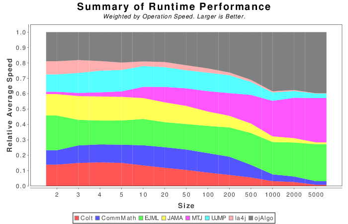
Summary box-and-whisker plots are an attempt to provide an overview of performance for all the libaries tested in a single plot. Higher numbers and more compact distributions represent better performance and more consistent performance across all operations, respectively.
The three bars represents performance across all matrix sizes, only the largest matrices, and only the smallest matrices. These Box-and-Whisker show the distribution relative of performance across all operations in a concise fashion. The thick rectangle in the middle contain the percentile results between 25% and 75%, the bar in the middle is the median, the dot is the mean, t-bar bounds the min and max values without the outliers, and dots represent outliers. The meaning of the triangles/arrows above and below is not known, JFreeChart does not specify, but it is suspected that they indicate more extreme outliers. If anyone knows what those triangles mean feel free to leave a comment below.
Weighted results are shown to place a heavier emphasis on operations that are more computationally expensive. This is justified because slower operations are often the bottle neck in an application. The weight is computed using the following procedure:
- For each matrix size find SLOWEST_BY_SIZE: the runtime of the operation whose fastest library has the longest processing time.
- For each operation in each matrix size compute N_OP:
N_OP = MAX_SAMPLES*(fastest library runtime) / SLOWEST_BY_SIZE
- Then for each operation in each library add its runtime performance to the bin N_OP times.
MAX_SAMPLES is arbitrarily set to 100. For example: if EJML ran at 75% of the speed of the fastest library for addition for a matrix of size 10 and addition took 12% of the time to complete compared to the slowest operation for a matrix of size 10, then 0.75 would be added to EJML’s bin 12 times. The distribution of each library’s bin are what the bar and whiskers plot is computed from.
Understanding Relative Runtime Plots
Results are presented primarily using relative runtime plots. These plots show how fast one library runs relative to another library across a range of matrix sizes for a single operation. An example of such a plot is shown below:
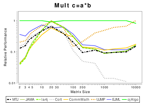
Higher numbers are better and represent more operations per second relative to other libraries. The scale is normalized against the fastest library at each matrix size. This formating is much succinct that standard FLOPS plots.
The x-axis is input matrix size and the y-axis shows the relative runtime. In general matrix size refers to the width and height of the input matrix/matrices, e.g. 100 on the axis refers to a 100 by 100 matrix with 10,000 elements. However there are some operations which use non-square matrices, see below. The reference library is the fastest library for each matrix size. Therefore one library always has a value of one. Larger the y-axis value is the faster the library is. If a plot ends prematurely for a library that means that it either became too slow or a fatal error occurred and the test was stopped.
By viewing these plots it is easy to tell how fast a particular library runs relative to any other library. Since these plots show the results as a function of matrix size it is often easy to see when CPU cache size starts adversely effecting one algorithm or when a library switches to a multi-threaded approach.
The benchmark also produces plots which show the absolute runtime. These have not been posted online for take of simplicity. Absolute runtime plots are in general more useful for understanding the behavior of an individual library and not for comparing performance across several libraries.
Absolute Runtime Plots

Absolute runtime plots show how long each operations takes. Unlike all the previous plots, lower numbers are better here.
In addition to relative runtime plots, plots of the absolute runtime are computed. These plots show on a log log scale how long each operation takes to run for each library. It is easier to see how the performance of each library changes as a function of time and how CPU caches affect it. However it is harder to see how much faster or slower each library is and these plots require more room to be clear.
For sake of simplicity absolute runtime plots are NOT included in the results pages. However they are automatically generated by the benchmark application.
Evaluated Operations
Three primary types of operations are tested; basic, solving, and decompositions. If a library did not support one of the operations it was simply omitted from that test.
Basic Operations
The following are several common operations used in linear algebra. There are many different permutations on these that some libraries support. For sake of brevity, only a few have been tested.
The transpose then multiply test is included to allow libraries that do not do a physical transpose to demonstrate their transpose performance. In general square matrices are used to avoid biasing the results towards an internal row-major or column-major format due to cpu caching issues.
| Operation | Description | Matrix Dimension |
|---|---|---|
| C = α * B | Scaling | B = (m x m) |
| C = A + B | Addition | A = (m x m), B=(m x m) |
| C = A * B | Matrix multiplication. | A = (m x m), B=(m x m) |
| C = AT * B | Transpose then multiplication | A = (m x m), B=(m x m) |
| det(A) | Determinant | A = (m x m) |
| C = AT | Physical transpose. | A = (m x m) |
| C = inv(A) | Invert. | A = (m x m) |
| C = symmInv(A) | Invert a symmetric matrix | A = (m x m) |
Linear Solving
Most libraries provided ways to solve for linear systems. Typically there are different algorithms used when a square system is being solved for versus an overdetermined system. Thus there are two benchmarks.
| Operation | Description | Matrix Dimension |
|---|---|---|
| x = A-1b where m=n | Solving for x when A is a square non-singular matrix. | A = (m x m), b = (m x 2m) |
| x = A-1b where m>n | Solving for x when it is an overdetermined system. | A = (3m x m), b = (3m x 2m |
Decompositions
For each of these operations the library is requested to perform the specified decomposition. Singular value and eigenvalue decompositions have the additional task of extracting the decomposed matrices. This additional task is done since for these decompositions the decomposed matrices are often of value to the user. In the other libraries raw matrices are used to solve or invert a system of equations.
| Operation | Description |
|---|---|
| SVD | Square matrix |
| Eigen | Symmetric square matrix |